Lab 1: Lambda Calculus

Review (10 minutes)

In other CS classes, we often consider how data (e.g., integers, strings, objects) can be represented as bits in memory. In $\lambda$-calculus, functions rather than bits are the primitive concepts, and the question becomes how can we encode/represent pieces of data as functions?

In class you saw some examples of encoding data as functions, e.g., encoding the boolean true value as the function (λx.(λy.x)) and the false value as the function (λx.(λy.y)).

Of course, not all $\lambda$-calculus functions are clever encodings of data; sometimes a function is just a function. For example, (λb. ((b False) True) is the one-argument boolean negation function. It takes a boolean value as input (encoded as a curried two-argument function) and uses the input to choose and return a boolean value (again encoded as a curried two-argument function).

Recall: Useful Concepts

$\beta$-reduction. This is the fundamental computation step in $\lambda$-calculus, where we apply a function to an argument. Examples include
```
     ((λx.x) a) → a
     ((λx.b) a) → b
     ((λx.(λy.x)) a) → (λy.a)
     ((λx.(λy.y)) a) → (λy.y)
```

Curried functions. We can encode multi-argument functions using functions that return functions, e.g.,

     (λx. ...)                 # a one-argument function
     (λx. (λy. ...))           # a two-argument function
     (λx. (λy. (λz. ...)))     # a three-argument function

     (f a)                     # applying a function to one argument
     ((f a) b)                 # applying a function to two arguments in succession
     (((f a) b) c)             # applying a function to three arguments in succession

Macro definitions. In class we defined abbreviations like

     True  := (λx.(λy.x));
     False := (λx.(λy.y));
     Pair  := (λx.(λy. (λb.((b x) y))));
     Fst   := (λp.(p True));
     Snd   := (λp.(p False));

(in class we drew a box around them rather than using the := symbol).

These are merely notational shorthand, letting us write

    (Fst ((Pair True) False))

instead of the much longer “official” form:

    ((λp.(p (λx.(λy.x)))) (((λx.(λy. (λb.((b x) y)))) (λx.(λy.x))) (λx.(λy.y))))

Getting the lab files (5 minutes)

For all labs, you will need to share a computer and work with a partner. There is no requirement that you will work with this partner (or any partner) on the homework assignment, or that you’ll have the same partner in future labs.

To get the lab files:

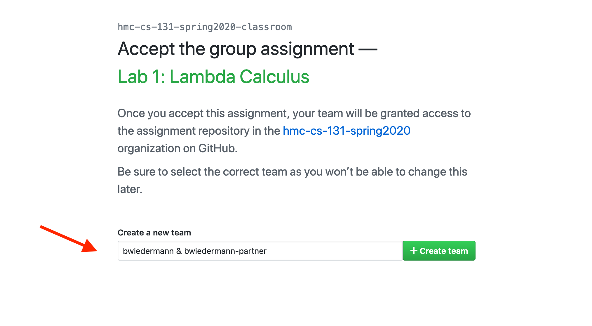
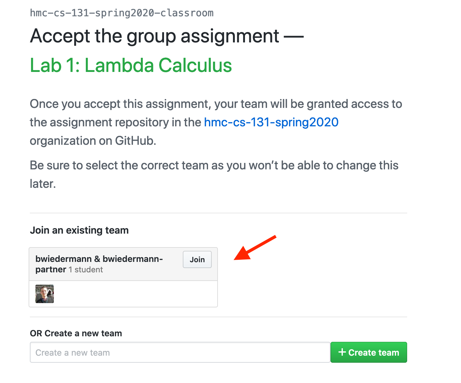
1. Create a team and accept the assignment.

One of the partners should go to the GitHub classroom link for the lab, provided on Piazza. Create a team name for your pair, based on the partners’ GitHub ids. Create a team based on your GitHub ids

Now the other partner should go to the GitHub classroom link for the lab. Find the newly created team and click the Join button. Join your partner's team

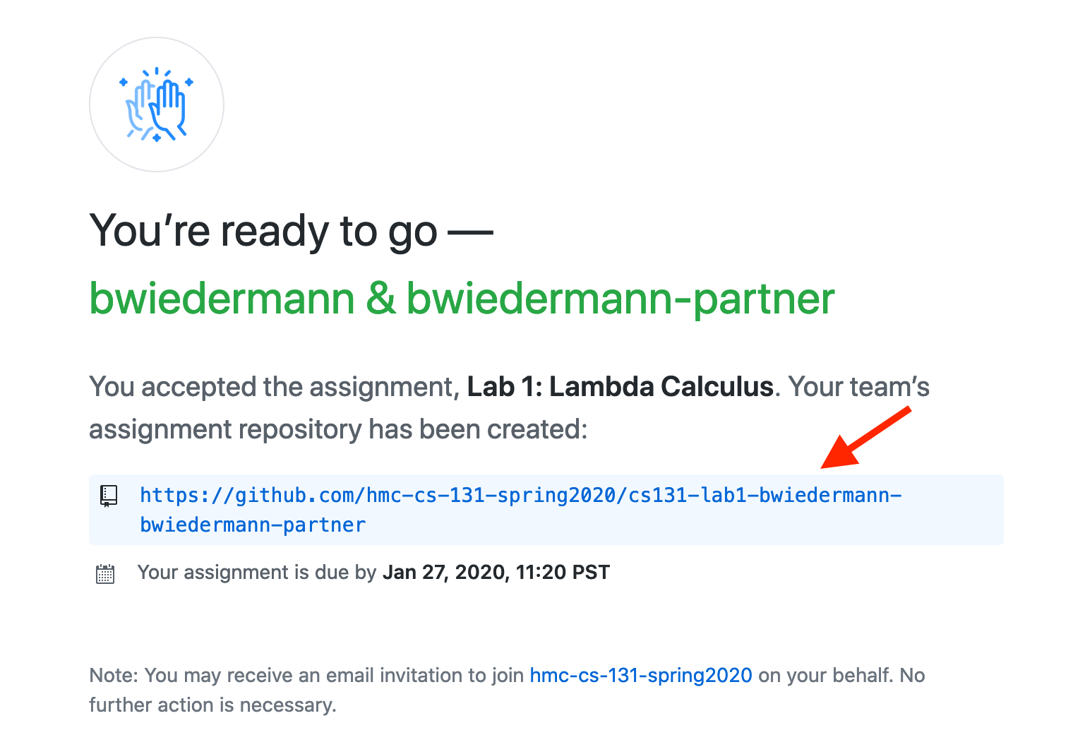
2. Clone the assignment repo to `knuth`.

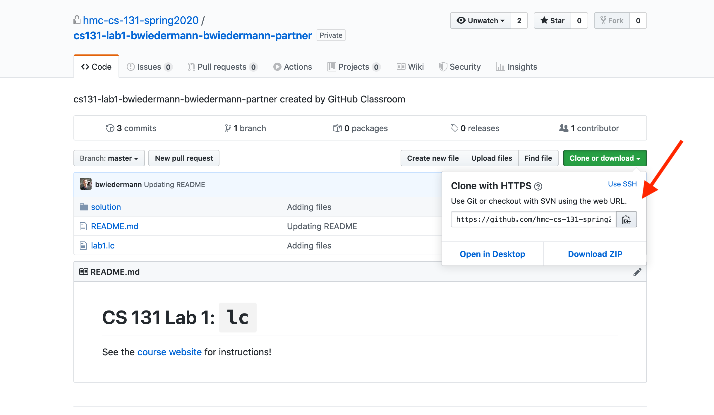
Once your repository has been created, one of the partners should:

Click on the link for the repository.
Click the Clone or download button and copy the URL.
Log into knuth and choose / make a directory to keep your files (e.g., ~/courses/cs131).
Change to that directory, e.g.,:
```
   cd ~/courses/cs131
```
In that directory, checkout the repository using the command
```
   git clone <url>
```
where <url> is the URL you copied in the previous step. You will probably be prompted for your GitHub id and password. After you enter them, the repository will be checked out in your directory on knuth.
Double-check that you have all the files by cding to the directory and using the ls command to list all the files:
```
    % cd cs131-lab1-bwiedermann-bwiedermann-partner
    % ls
    README.md  lab1.lc  solution
```

You will notice that the lab comes with a solution. We make the solution available so that you can check your progress after trying the lab. Resist looking unless and until you need a hint or confirmation that you are on the right track!

Running a $\lambda$-Calculus Interpreter (10 minutes)

There is a simple $\lambda$-calculus interpreter installed on the CS server knuth.cs.hmc.edu. You can run it by ssh-ing to knuth.cs.hmc.edu and invoking lc at the command line. As shown in the following transcript of two inputs, lc defaults to showing the reduction steps it performs:

                lc> ((\x.x) y)

                After 0 β-reductions:

                    ((λx.x) y)
                  →β
                    y

                1 total steps

                lc> (((\x.(\y.(y x))) (\z.(z z))) (\w.w))

                After 0 β-reductions:

                    (((λx.(λy.(y x))) (λz.(z z))) (λw.w))
                  →β
                    ((λy.(y (λz.(z z)))) (λw.w))

                After 1 β-reductions:

                    ((λy.(y (λz.(z z)))) (λw.w))
                  →β
                    ((λw.w) (λz.(z z)))

                After 2 β-reductions:

                    ((λw.w) (λz.(z z)))
                  →β
                    (λz.(z z))

                3 total steps

Start lc on Knuth and try a couple of lambda expressions, such as the ones above, or others of your choosing. Notice that each step shows the expression before the beta reduction and afterwards (using underlining to show where the beta-reduction happened, and using colors to show how the argument was substituted into the function).

To make typing easier, instead of (λx.x) you can write (\x.x) in the input. (A backslash is the best we can do in ASCII; at least it’s “two thirds of a lambda”).
Enter :help to see the built-in commands, and try re-running some of the same expressions with different amounts of tracing. (If you use up/down-arrow or control-p/n to scroll through the input history, you don’t have to re-type everything.)
Set the trace level back to full and load the given files by saying:
```
     :set trace full
     :load lab1.lc
```
These commands load the macros defined in the file lab1.lc (including True, False, Not, And, Or, Pair, Fst, Snd).
In lc, evaluate ((And ((Or True) False)) ((And True) True))

Scroll back upwards in the terminal to where you typed the command and read over the output as it performs reductions. Notice the way the output is color-coded to show what function is being applied and its argument, and where the argument goes after substitution is complete.

You’ll notice from the output that lc does not expand macros until it is forced to, making the output more readable. Try a few other inputs such as ((True False) True) or (Fst ((Pair True) False)). Confirm that the answers are what you expect.

Open the knuth version of `lab1.lc` in an editor. (5 minutes)

The simplest way to edit the lab1.lc file is to use Visual Studio + Remote SSH. Once you have connected to knuth, open the folder that contains your repository files.

(Another option is to create a separate terminal window and/or ssh connection to Knuth, and run a text-mode editor there, so that you can have the editor and the lc program running and visible simultaneously. There are several text-mode editors on Knuth, such as nano, emacs, and vim.)

(Another option, you can ssh with the -Y flag (i.e., ssh -Y «username»@knuth.cs.hmc.edu). Then as long as your computer has XQuartz (for Macs, available at www.xquartz.org) or some other X-Windows server installed, you can run programs on Knuth that display their GUI locally on your laptop. Editors on Knuth that support graphical display include gedit, xemacs, and gvim.)

Look over the lab1.lc file in your editor. There should be no real surprises, but notice that macro names are always capitalized, variables are always lowercase, and there are semicolons at the end of macro definitions.

Encoding lists (version 1)

By definition, a list is either empty or it has a head (first element) and a tail (a list containing the rest of the elements, possibly empty).

To represent lists in $\lambda$-calculus, we want a lambda expression Nil to represent the empty list, and a function Cons such that ((Cons hd) tl) represents the non-empty list with head hd and with tail tl. For example

        Nil                            # encodes []
        ((Cons s) Nil)                 # encodes [s]
        ((Cons r) ((Cons s) Nil))      # encodes [r,s]

There are many, many possible ways to encode lists. The file lab1.lc defines Cons and Nil using a fairly simplistic scheme involving pairs and booleans.

Define the following functions in lab1.lc to work with this encoding:

The function IsNil should return True if given the (encoded) list Nil and return False if given a non-empty list (i.e., it should return False if given a list encoded using the Cons function).
The function Head should return the head of a list that was constructed using Cons.
The function Tail should return the tail of a list that was constructed using Cons.

Reload your definitions into lc and verify that for all h and t:

(IsNil ((Cons h) t)) reduces to False.
(Head ((Cons h) t)) reduces to h
(Tail ((Cons h) t)) reduces to t

Arithmetic with Church Numerals

The Church numerals are curried functions that encode nonnegative integers:

:= (λf.(λb. b));
:= (λf.(λb. (f b)));
:= (λf.(λb. (f (f b))));
:= (λf.(λb. (f (f (f b)))));
:= (λf.(λb. (f (f (f (f b))))));
    ...etc...

Church numerals give us the ability to do something a fixed number of times. For example, the Church numeral for 2 gives us the ability to apply any function twice: for any function g and initial value v, the expression ((2 g) v) applies g twice, starting with v, like so: (g (g v)). Similarly ((7 g) v) applies g seven times, starting with v and returns the result. In general, if n is some Church numeral encoding the number $n$, then ((n g) v) applies g $n$ times, starting with v.

To show that Church numerals really encode numbers, we can define Succ, the successor or “add one” function. If n is a Church numeral then ((n f) b) applies f to b $n$ times and returns the result; thus (f ((n f) b)) applies f to b $n$ times and then once more, for a total of $n{+}1$ times. That justifies the definition of successor:

    Succ := (\n. (\f.(\b. (f ((n f) b)))));

Successor

Verify using lc that (Succ 0), (Succ 1), and (Succ 6) all produce the correct answers.

Addition

Define Plus in lab1.lc. Reload your definitions into lc and verify that it works. For example, ((Plus 2) 2) should reduce to the Church numeral for 4. Remember:

In $\lambda$-calculus, two-argument functions like Plus are defined as curried functions (functions that return functions).
Having a Church numeral i gives you the ability to do anything $i$ times to something; just apply i to two arguments in succession: once to the operation you want to repeat, and once to the starting value.
Adding $m$ to $n$ is like applying the successor function, repeated $m$ times, starting at $n$.

Multiplication

Come up with a working definition for Times in lab1.lc. Verify that it works, e.g., that ((Times 3) 2) reduces to the Church numeral 6. Hints:

Multiplying $m$ by $n$ is like adding $m$, repeated $n$ times, starting at $0$.
This suggests we need a one-argument “add m” function.

`IsZero`

IsZero is kind of fun. Given a Church numeral (the ability to apply a function $n$ times), we want to know whether $n$ is $0$ or not. We can do this by applying the ignore-the-argument-and-return-False function (λx.False), and apply it $n$ times to the value True.

if $n = 0$ then we apply the function zero times to True, resulting in True;
if $n = 1$ then we apply the function one time to True, resulting in False;
if $n = 2$ then we apply the “return False” function twice to True, resulting in False;
and so on.

IsZero has been defined for you. Verify that (IsZero 0), (IsZero 1), and (IsZero 7) reduce as expected.

Predecessor

Pred is the most challenging numerical function to write. You can’t “unapply” a function, so you can’t easily turn 10 (the ability to apply any function 10 times) into 9 (the ability to apply any function 9 times).

A clever insight (due to logician Stephen Kleene) starts with the following sequence of pairs:

((Pair 0) 0)
((Pair 0) 1)
((Pair 1) 2)
((Pair 2) 3)
((Pair 3) 4)
...

Notice that:

There is fixed rule to turn each pair into the next: (a,b) turns into (b, b+1).
If we take ((Pair 0) 0) and apply that rule n times, we get the $n$-th pair in the sequence, whose first component is $n-1$. (We don’t have negative Church numerals, so we have to define 0 to be its own predecessor.)

You are given the code

    Pred = (λn. (Fst ((n NextPair) ((Pair 0) 0))));

that follows the above recipe: given $n$, apply NextPair, repeated $n$ times, to the pair $(0,0)$, resulting in the $n$-th pair in the sequence; finally, extract the pair’s first component to get $n{-}1$.

However, the function NextPair (which takes as input a pair p in the sequence and returns the next pair in the sequence) is incomplete. Finish this definition, and verify that, e.g., (Pred 3) is the Church numeral 2.

Subtraction

Just as we defined addition as repeated successor, we can define subtraction as repeated predecessor. This definition yields a version of subtraction which cannot go strictly negative; subtracting a large number from a small number just returns 0. This definition is provided for you in lab1.lc; since it’s not quite true subtraction—we can’t go negative—the operation has the special name Monus.

Verify that ((Monus 4) 2) produces 2, but ((Monus 2) 4) produces 0. Subtractions involving large numbers require a lot more $\beta$-reduction steps than additions do. Can you explain why they are so expensive?

Submit your work

When you are done (or at the end of the lab period, whichever comes first), follow the assignment workflow to push your changes from knuth to GitHub.

After the changes are pushed, one of the partners should submit your lab work on Gradescope. Be sure to add your partner after submitting!. Add your team member to your Gradescope submission